Module 7
Updated 2021/05/07
The Book of R: chapter 7.1, 7.2 (plots), ?system2
Module 6 review
Built in functions
mysum = function(arg1) {
return (sum(arg1))
}
Regular expressions
- b[ce]+d
- b[ce]*d
Exercise: A useful function (10 minutes)
Following on from the previous exercise where you found a string matching a regular expression…
Write a function that returns all the matches of a regular expression in a string
Hint: use substring (not substr) – why?
Test that the function works in the same way as in the previous exercise (by searching DNA for G..A)
Exercise solution (5 minutes)
DNA <- "ACGATGATACTGATGACGGGCGCCA"
REGEX <- "G..A"

# figuring things out ----
matches <- gregexpr(REGEX,DNA)[[1]]
substr(
  DNA,
  matches,
  matches + attr(matches,"match.length") - 1
)
## [1] "GATA"substring(
DNA,
matches,
matches + attr(matches,"match.length") - 1
)## [1] "GATA" "GCCA"# the function ----
MATCHER <- function(STRING,REGEX) {
matches <- gregexpr(REGEX,DNA)[[1]]
return(substring(
DNA,
matches,
matches + attr(matches,"match.length") - 1
))
}
MATCHER(DNA,REGEX)## [1] "GATA" "GCCA"Interfacing with external programs
- You can call/execute an external program from within your script
- Helps you automate certain tasks that would be difficult for you to do within R e.g. useful programs that are not available in R
# system2() #calls an external command
system2("ls")  #unix/mac
## Warning in system2("ls"): '"ls"' not foundsystem2("cmd.exe", input="dir") #windowssystem2 function
#returns stdout in variable v
v = system2("ls", stdout=T)
v

#passes arguments to the command (ls)
v = system2("ls", args="-la", stdout=T)
v- What’s wrong with system()?
- It works, but is older and not recommended
Exercise: external programs (10 minutes)
Write a script to call a system command
- Mac/unix users
- Run the “df –h” UNIX command from the shell – what does it do?
- Call “df -h” from R to see how much space is left on your hard drive
- Check your results against the “df -h” command you ran
- Windows users
- Try to run windows “time” or “dir” commands
- E.g. system2(“cmd.exe”, input=“dir”)
- Can also try shell(“dir”)
Exercise solution (5 minutes)
# This was knit on a Windows OS:
try({
  system2("ls",stdout=T)
},silent=F)
## Error in system2("ls", stdout = T) : '"ls"' not foundsystem2(command="cmd.exe",input="dir",stdout=T)## [1] "Microsoft Windows [Version 10.0.19042.985]"
## [2] "(c) Microsoft Corporation. All rights reserved."
## [3] ""
## [4] "D:\\Dropbox\\TA_MMG1002H_2020\\p4b>dir"
## [5] " Volume in drive D is DATA"
## [6] " Volume Serial Number is 36E0-89E7"
## [7] ""
## [8] " Directory of D:\\Dropbox\\TA_MMG1002H_2020\\p4b"
## [9] ""
## [10] "2021-05-31 12:54 PM <DIR> ."
## [11] "2021-05-31 12:54 PM <DIR> .."
## [12] "2020-04-23 09:49 AM 44 .gitignore"
## [13] "2021-05-28 12:54 PM 19,299 .Rhistory"
## [14] "2021-04-30 01:41 PM 30 aaoutput.txt"
## [15] "2019-03-04 12:05 AM 653,001 ASCII-Table-wide.svg"
## [16] "2021-04-30 01:30 PM 218 assignment2_sequence.txt"
## [17] "2021-05-31 12:54 PM 58,595 column.txt"
## [18] "2021-05-31 12:54 PM <DIR> docs"
## [19] "2019-03-03 11:44 PM 66,773 fileOutput.png"
## [20] "2021-04-23 12:58 PM 1,010,056 gene_condition_source_id.txt"
## [21] "2021-05-10 01:36 PM 2,263,040 GSE13924_RAW.tar"
## [22] "2008-12-15 03:34 PM 1,173,030 GSM350771.CEL.gz"
## [23] "2008-12-15 03:34 PM 1,078,395 GSM350772.CEL.gz"
## [24] "2021-05-31 12:54 PM 10,159 index.html"
## [25] "2021-05-03 08:43 AM 241 index.md"
## [26] "2021-05-31 12:54 PM 20,372 mod1.html"
## [27] "2021-04-23 12:58 PM 6,249 mod1.Rmd"
## [28] "2021-05-31 12:54 PM 31,365 mod2.html"
## [29] "2021-04-19 02:31 PM 10,003 mod2.Rmd"
## [30] "2021-05-31 12:54 PM 15,510 mod2.utf8.md"
## [31] "2021-05-31 12:54 PM <DIR> mod2_files"
## [32] "2021-05-31 12:54 PM 29,603 mod3.html"
## [33] "2021-04-23 02:45 PM 5,908 mod3.Rmd"
## [34] "2021-05-31 12:54 PM 39,502 mod4.html"
## [35] "2021-04-30 01:13 PM 11,181 mod4.Rmd"
## [36] "2021-05-31 12:54 PM 38,416 mod5.html"
## [37] "2021-04-30 04:14 PM 17,749 mod5.Rmd"
## [38] "2021-05-31 12:54 PM 22,342 mod5.utf8.md"
## [39] "2021-04-30 04:02 PM 469 mod5exercise.fa"
## [40] "2021-05-31 12:54 PM 24,709 mod6.html"
## [41] "2021-05-31 12:54 PM 11,871 mod6.knit.md"
## [42] "2021-05-03 03:19 PM 8,566 mod6.Rmd"
## [43] "2021-05-31 12:54 PM 11,871 mod6.utf8.md"
## [44] "2021-05-31 12:54 PM 34,072 mod7.knit.html"
## [45] "2021-05-07 04:47 PM 19,265 mod7.knit.md"
## [46] "2021-05-07 04:43 PM 6,928 mod7.Rmd"
## [47] "2021-05-10 02:31 PM 10,087 mod8.Rmd"
## [48] "2021-05-14 02:30 PM 7,717 mod9.Rmd"
## [49] "2021-05-14 02:30 PM 29,505 mod9.utf8.md"
## [50] "2021-05-31 12:54 PM 17,815 mod_me.html"
## [51] "2021-05-31 12:54 PM 5,381 mod_me.Rmd"
## [52] "2021-05-31 12:54 PM <DIR> mod_me_files"
## [53] "2021-05-31 12:54 PM 96 mydata.txt"
## [54] "2021-05-31 11:42 AM 240 p4b.Rproj"
## [55] "2020-04-23 10:52 AM 184 README.md"
## [56] "2019-03-03 10:12 PM 522,169 recipebookTOC.png"
## [57] "2021-05-31 12:54 PM 74 row.txt"
## [58] "2021-04-30 03:19 PM 57,680 RStudioOptions.png"
## [59] "2021-05-31 12:54 PM <DIR> site_libs"
## [60] "2021-04-16 02:41 PM 218 sum.R"
## [61] "2021-05-10 02:31 PM 277,911 test.txt"
## [62] "2021-05-14 02:12 PM 4,972 thisisapdf.pdf"
## [63] "2021-05-14 02:14 PM 28,850 thisisnotapdf.png"
## [64] "2011-11-18 12:42 AM 291,755 yeast_properties.txt"
## [65] "2021-05-31 12:34 PM 667 _site.yml"
## [66] " 50 File(s) 7,954,153 bytes"
## [67] " 6 Dir(s) 280,114,880,512 bytes free"
## [68] ""
## [69] "D:\\Dropbox\\TA_MMG1002H_2020\\p4b>"shell("ls",shell="bash")
shell("df -h",shell="bash")Recipes
Code examples and templates
- Recipes are standard way to do things
- Look up the recipes in a cookbook
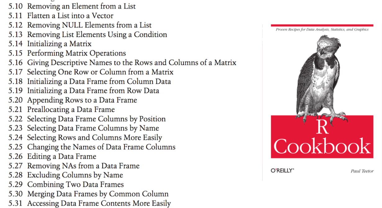
R recipe book
Example recipes
#Sorting a data frame
data_frame = data_frame[order(data_frame$key) , ]
#data_frame$key is the column to sort by
#Note: the sort() function only works for vectors, not data frames

#Sorting by two columns
data_frame = data_frame[order(data_frame$key1,data_frame$key2) , ]
#The second key is used to break ties in the first

#Removing elements from a list
#Set the value to be NULL
Stack Overflow
- User-contributed question and answer website – good free source of recipes
- e.g. How to delete multiple values from a vector?
Plots
Graphically plotting/charting data
Introduction to plots
#R has powerful data plotting abilities
hist(runif(50))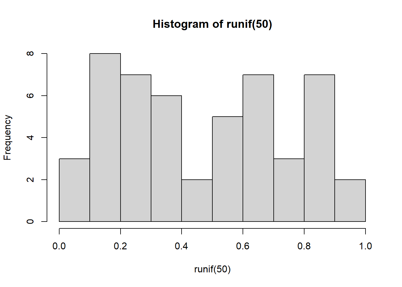
plot(runif(50))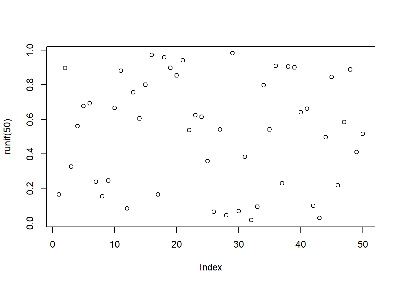
plot(runif(50), runif(50)) #x,y scatter plot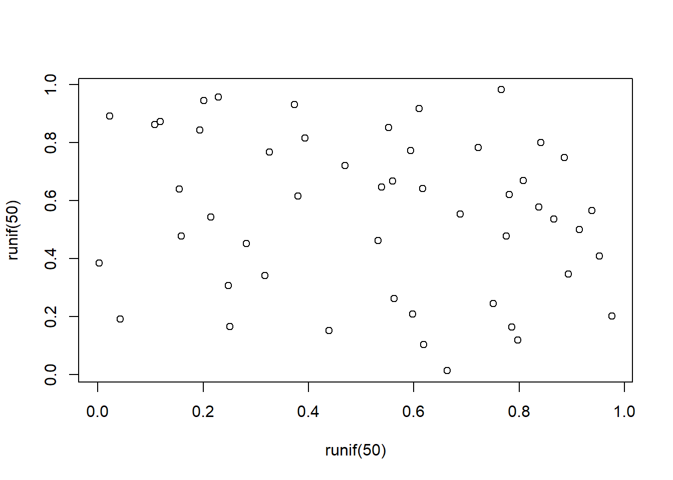
boxplot(runif(50))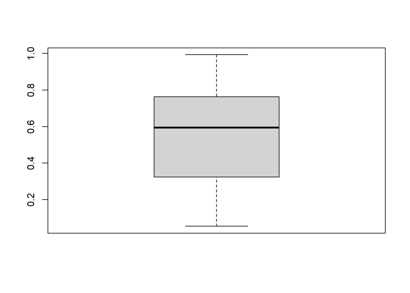
demo(graphics)##
##
## demo(graphics)
## ---- ~~~~~~~~
##
## > # Copyright (C) 1997-2009 The R Core Team
## >
## > require(datasets)
##
## > require(grDevices); require(graphics)
##
## > ## Here is some code which illustrates some of the differences between
## > ## R and S graphics capabilities. Note that colors are generally specified
## > ## by a character string name (taken from the X11 rgb.txt file) and that line
## > ## textures are given similarly. The parameter "bg" sets the background
## > ## parameter for the plot and there is also an "fg" parameter which sets
## > ## the foreground color.
## >
## >
## > x <- stats::rnorm(50)
##
## > opar <- par(bg = "white")
##
## > plot(x, ann = FALSE, type = "n")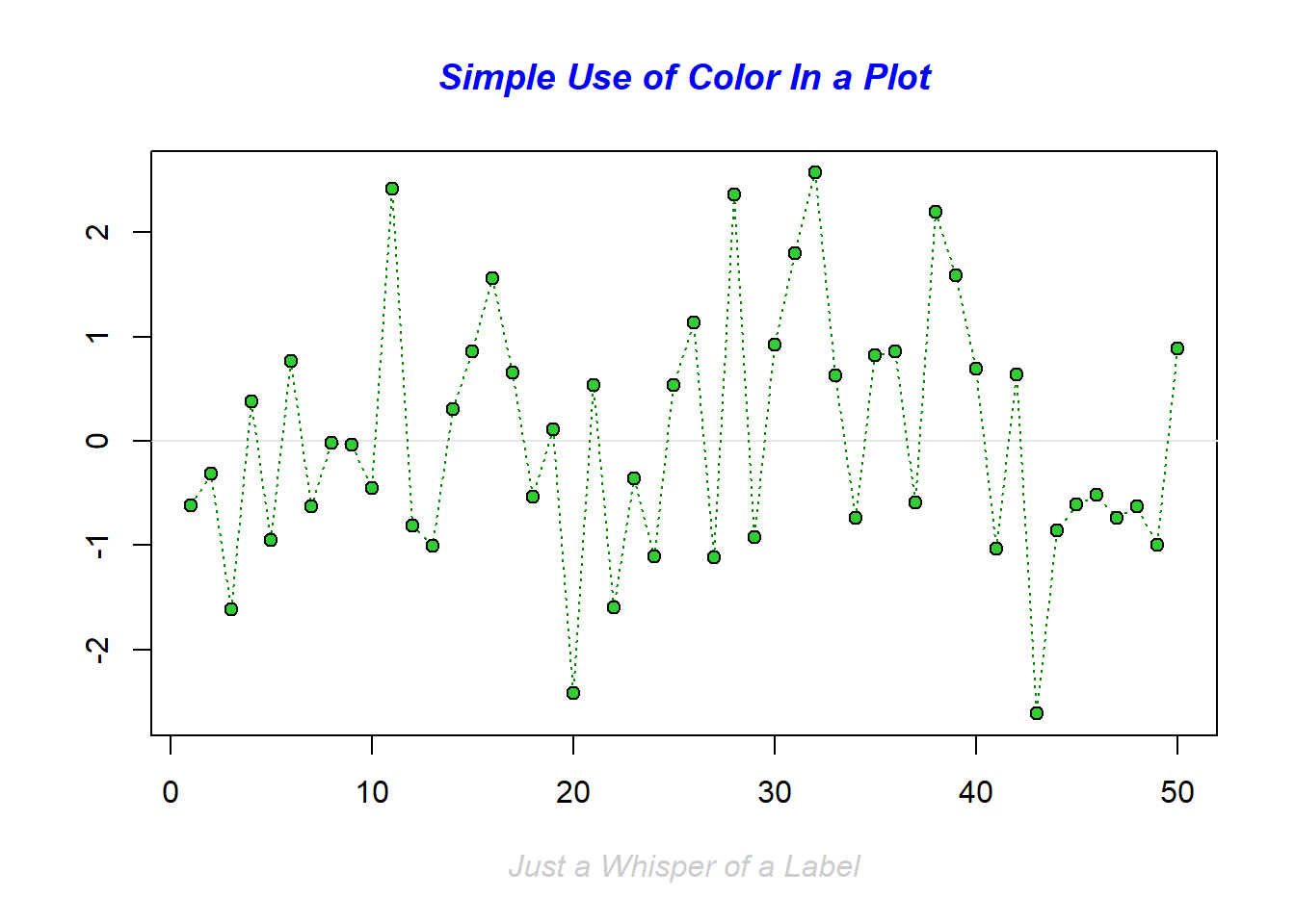
##
## > abline(h = 0, col = gray(.90))
##
## > lines(x, col = "green4", lty = "dotted")
##
## > points(x, bg = "limegreen", pch = 21)
##
## > title(main = "Simple Use of Color In a Plot",
## +       xlab = "Just a Whisper of a Label",
## +       col.main = "blue", col.lab = gray(.8),
## +       cex.main = 1.2, cex.lab = 1.0, font.main = 4, font.lab = 3)
##
## > ## A little color wheel.    This code just plots equally spaced hues in
## > ## a pie chart.    If you have a cheap SVGA monitor (like me) you will
## > ## probably find that numerically equispaced does not mean visually
## > ## equispaced.  On my display at home, these colors tend to cluster at
## > ## the RGB primaries.  On the other hand on the SGI Indy at work the
## > ## effect is near perfect.
## >
## > par(bg = "gray")
##
## > pie(rep(1,24), col = rainbow(24), radius = 0.9)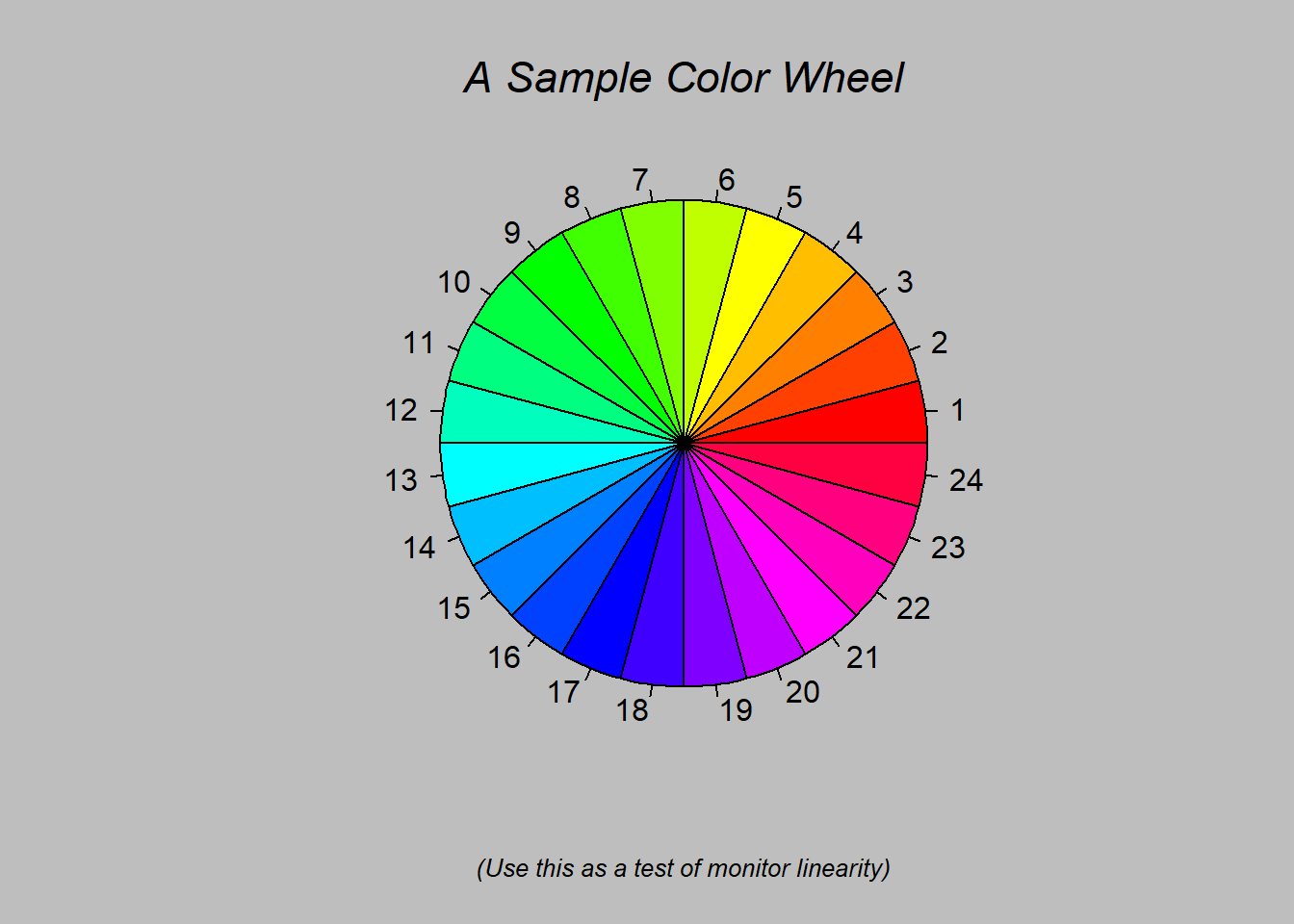
##
## > title(main = "A Sample Color Wheel", cex.main = 1.4, font.main = 3)
##
## > title(xlab = "(Use this as a test of monitor linearity)",
## +       cex.lab = 0.8, font.lab = 3)
##
## > ## We have already confessed to having these.  This is just showing off X11
## > ## color names (and the example (from the postscript manual) is pretty "cute".
## >
## > pie.sales <- c(0.12, 0.3, 0.26, 0.16, 0.04, 0.12)
##
## > names(pie.sales) <- c("Blueberry", "Cherry",
## +              "Apple", "Boston Cream", "Other", "Vanilla Cream")
##
## > pie(pie.sales,
## +     col = c("purple","violetred1","green3","cornsilk","cyan","white"))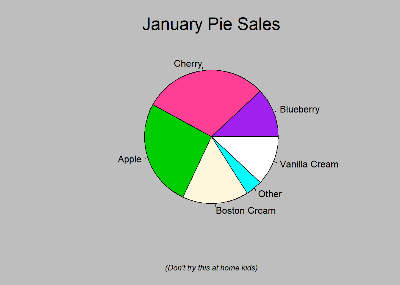
##
## > title(main = "January Pie Sales", cex.main = 1.8, font.main = 1)
##
## > title(xlab = "(Don't try this at home kids)", cex.lab = 0.8, font.lab = 3)
##
## > ## Boxplots:  I couldn't resist the capability for filling the "box".
## > ## The use of color seems like a useful addition, it focuses attention
## > ## on the central bulk of the data.
## >
## > par(bg="cornsilk")
##
## > n <- 10
##
## > g <- gl(n, 100, n*100)
##
## > x <- rnorm(n*100) + sqrt(as.numeric(g))
##
## > boxplot(split(x,g), col="lavender", notch=TRUE)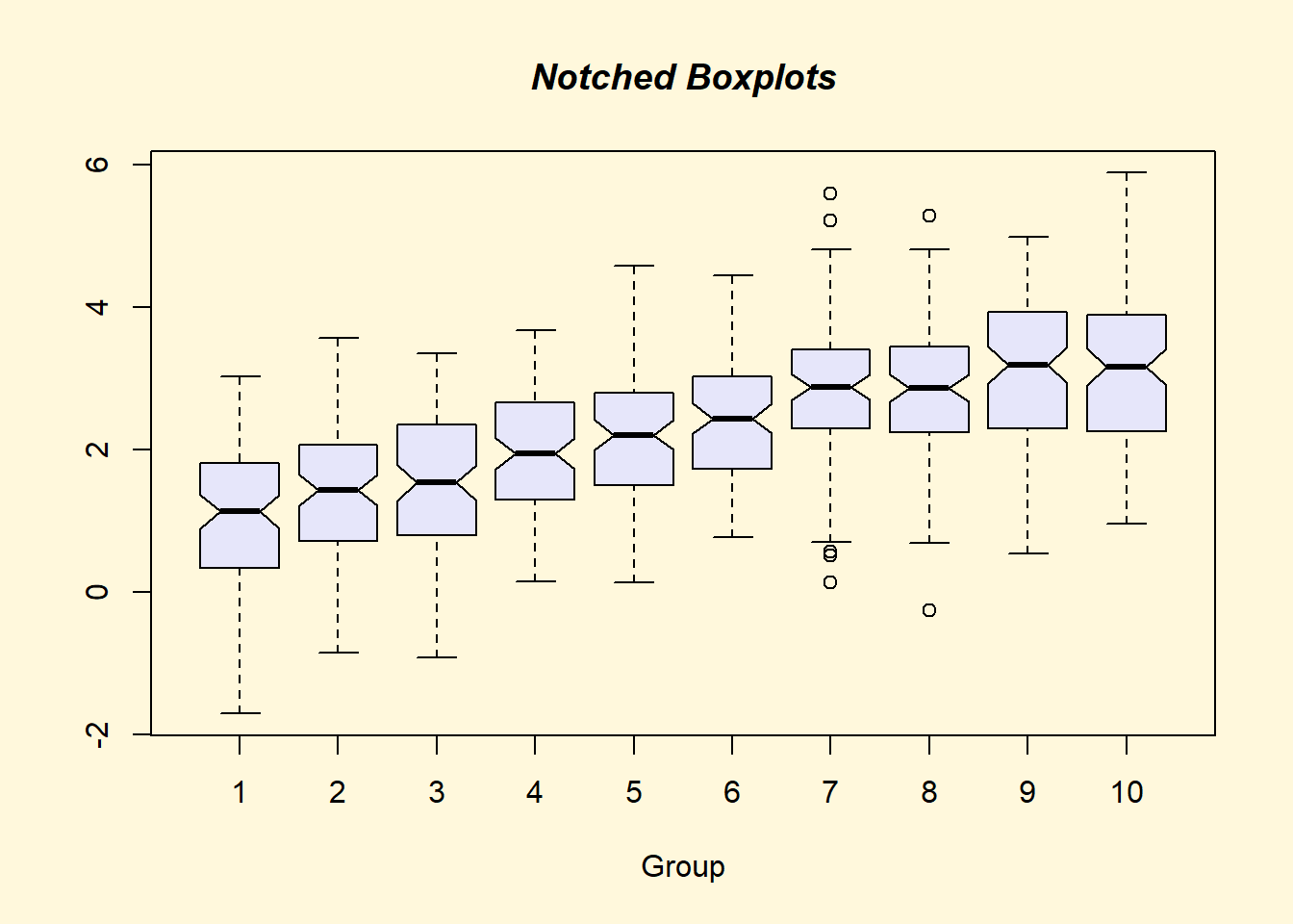
##
## > title(main="Notched Boxplots", xlab="Group", font.main=4, font.lab=1)
##
## > ## An example showing how to fill between curves.
## >
## > par(bg="white")
##
## > n <- 100
##
## > x <- c(0,cumsum(rnorm(n)))
##
## > y <- c(0,cumsum(rnorm(n)))
##
## > xx <- c(0:n, n:0)
##
## > yy <- c(x, rev(y))
##
## > plot(xx, yy, type="n", xlab="Time", ylab="Distance")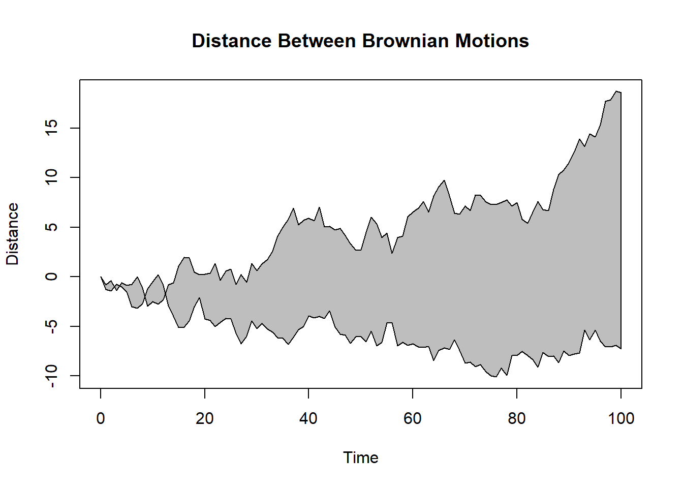
##
## > polygon(xx, yy, col="gray")
##
## > title("Distance Between Brownian Motions")
##
## > ## Colored plot margins, axis labels and titles.    You do need to be
## > ## careful with these kinds of effects.    It's easy to go completely
## > ## over the top and you can end up with your lunch all over the keyboard.
## > ## On the other hand, my market research clients love it.
## >
## > x <- c(0.00, 0.40, 0.86, 0.85, 0.69, 0.48, 0.54, 1.09, 1.11, 1.73, 2.05, 2.02)
##
## > par(bg="lightgray")
##
## > plot(x, type="n", axes=FALSE, ann=FALSE)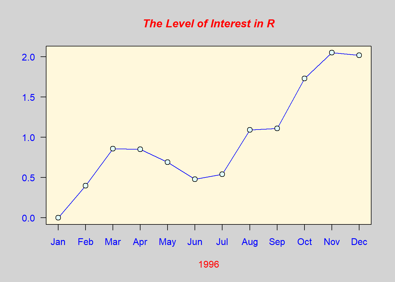
##
## > usr <- par("usr")
##
## > rect(usr[1], usr[3], usr[2], usr[4], col="cornsilk", border="black")
##
## > lines(x, col="blue")
##
## > points(x, pch=21, bg="lightcyan", cex=1.25)
##
## > axis(2, col.axis="blue", las=1)
##
## > axis(1, at=1:12, lab=month.abb, col.axis="blue")
##
## > box()
##
## > title(main= "The Level of Interest in R", font.main=4, col.main="red")
##
## > title(xlab= "1996", col.lab="red")
##
## > ## A filled histogram, showing how to change the font used for the
## > ## main title without changing the other annotation.
## >
## > par(bg="cornsilk")
##
## > x <- rnorm(1000)
##
## > hist(x, xlim=range(-4, 4, x), col="lavender", main="")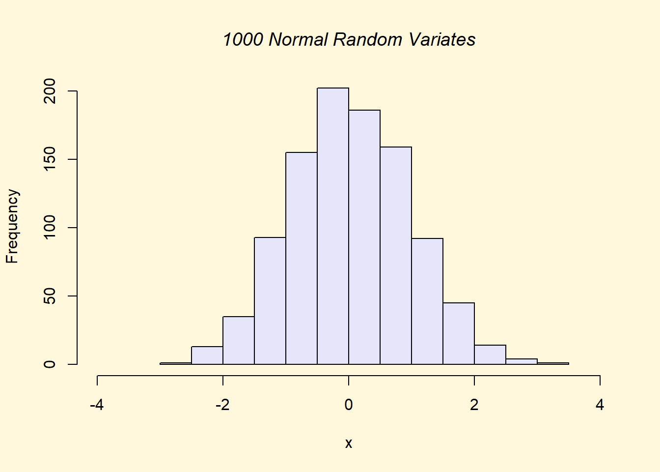
##
## > title(main="1000 Normal Random Variates", font.main=3)
##
## > ## A scatterplot matrix
## > ## The good old Iris data (yet again)
## >
## > pairs(iris[1:4], main="Edgar Anderson's Iris Data", font.main=4, pch=19)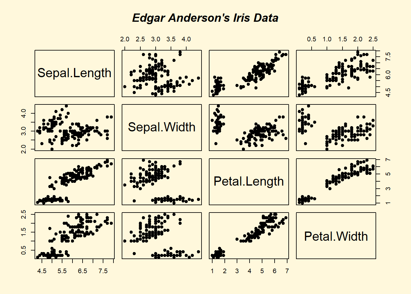
##
## > pairs(iris[1:4], main="Edgar Anderson's Iris Data", pch=21,
## +       bg = c("red", "green3", "blue")[unclass(iris$Species)])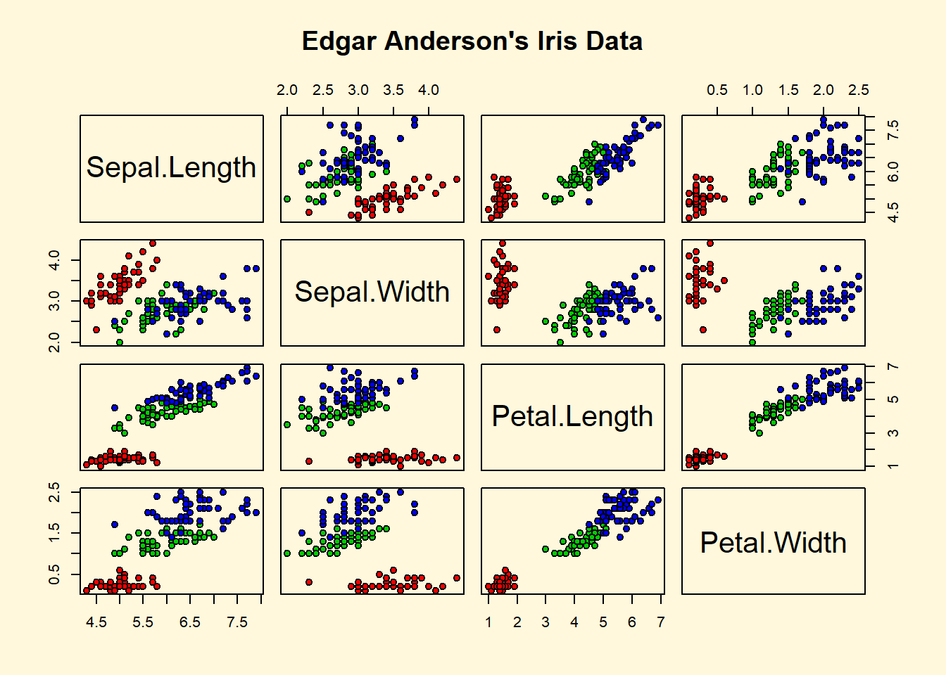
##
## > ## Contour plotting
## > ## This produces a topographic map of one of Auckland's many volcanic "peaks".
## >
## > x <- 10*1:nrow(volcano)
##
## > y <- 10*1:ncol(volcano)
##
## > lev <- pretty(range(volcano), 10)
##
## > par(bg = "lightcyan")
##
## > pin <- par("pin")
##
## > xdelta <- diff(range(x))
##
## > ydelta <- diff(range(y))
##
## > xscale <- pin[1]/xdelta
##
## > yscale <- pin[2]/ydelta
##
## > scale <- min(xscale, yscale)
##
## > xadd <- 0.5*(pin[1]/scale - xdelta)
##
## > yadd <- 0.5*(pin[2]/scale - ydelta)
##
## > plot(numeric(0), numeric(0),
## +      xlim = range(x)+c(-1,1)*xadd, ylim = range(y)+c(-1,1)*yadd,
## +      type = "n", ann = FALSE)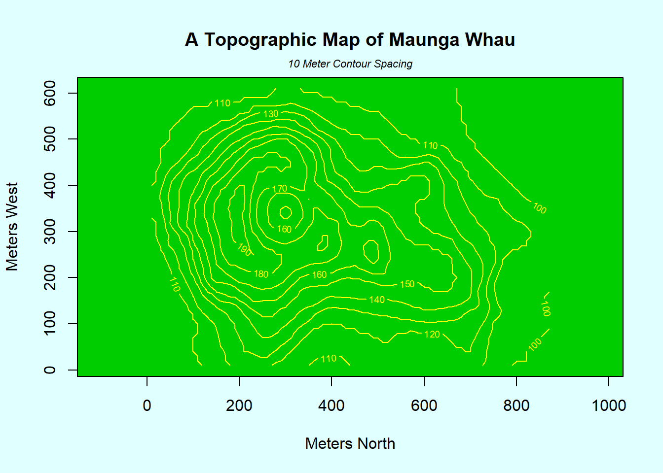
##
## > usr <- par("usr")
##
## > rect(usr[1], usr[3], usr[2], usr[4], col="green3")
##
## > contour(x, y, volcano, levels = lev, col="yellow", lty="solid", add=TRUE)
##
## > box()
##
## > title("A Topographic Map of Maunga Whau", font= 4)
##
## > title(xlab = "Meters North", ylab = "Meters West", font= 3)
##
## > mtext("10 Meter Contour Spacing", side=3, line=0.35, outer=FALSE,
## +       at = mean(par("usr")[1:2]), cex=0.7, font=3)
##
## > ## Conditioning plots
## >
## > par(bg="cornsilk")
##
## > coplot(lat ~ long | depth, data = quakes, pch = 21, bg = "green3")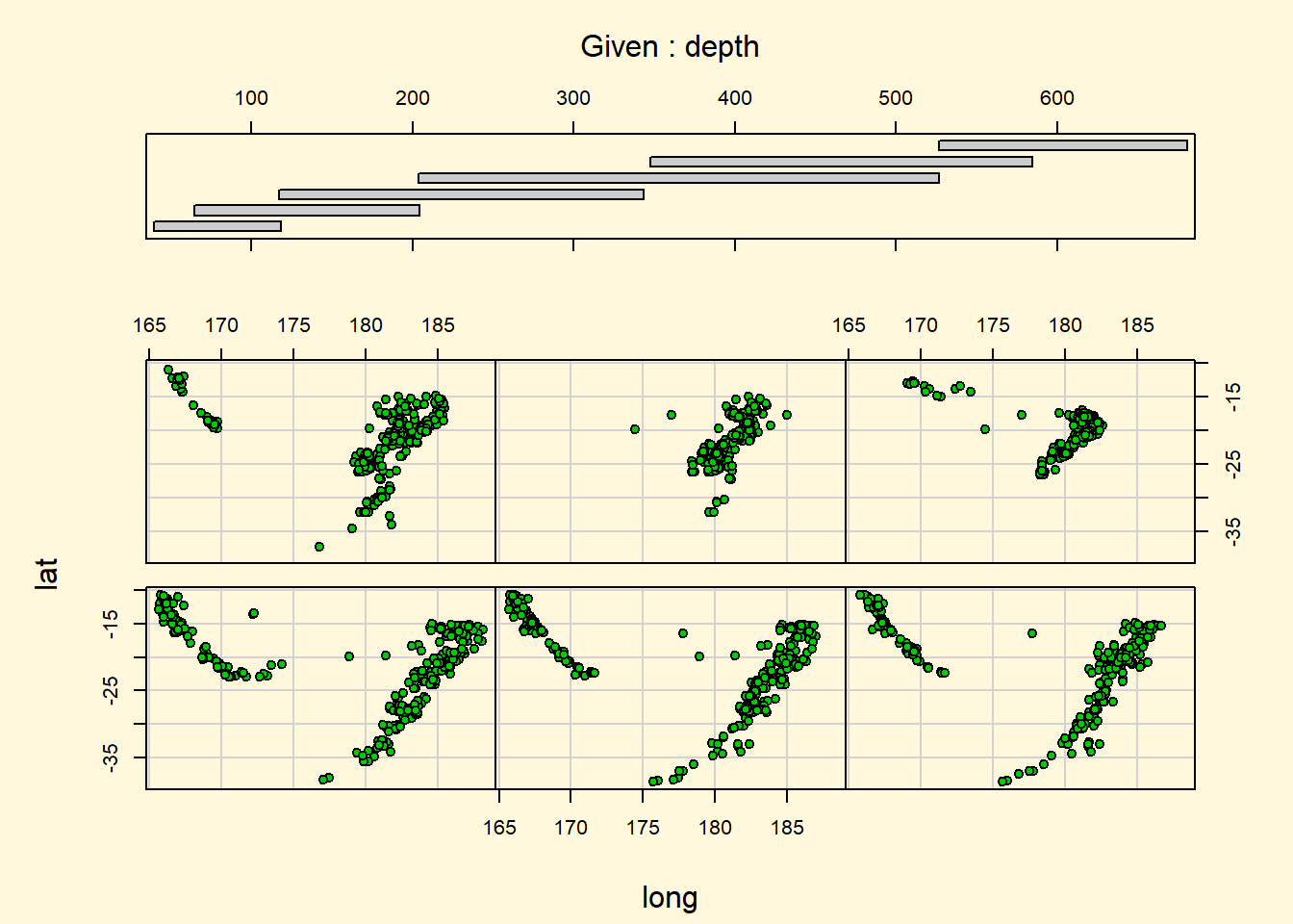
##
## > par(opar)
Exercise: plots (10 minutes)
Create a matrix “randomdata” with 50 rows and 10 columns using “replicate(10,rnorm(50))”
Plot the first and second columns of the matrix in a scatter plot
Generate a vector “randommeans” with the means of all columns of randomdata. Also generate a vector “randomsds” with the standard deviations of all columns of randomdata
Generate a boxplot of the first and second columns of randomdata
Exercise solution (5 minutes)
# Make random (normal!) data ----
randomdata1 <- matrix(rnorm(500),nrow=50,ncol=10)
randomdata2 <- replicate(10,rnorm(50))
#^ is a wrapper for sapply(1:10,function(X) rnorm(50))

temp <- list()
for(i in 1:10) {
  temp[[i]] <- rnorm(50)
}
randomdata3 <- do.call("cbind",temp)

dim(randomdata1)
## [1] 50 10str(randomdata2)## num [1:50, 1:10] 0.486 1.273 -0.171 0.423 0.512 ...str(randomdata3)## num [1:50, 1:10] 0.92 0.932 1.337 -0.418 0.996 ...# step 2 ----
default_par <- par(no.readonly=T)
par(mfrow=c(1,3),mar=c(3,3,1,1),mgp=c(2,1,0))
plot(randomdata1[,1:2])
plot(x=randomdata1[,1],y=randomdata1[,2])
rd4 <- as.data.frame(randomdata1)
plot(V2~V1,data=rd4)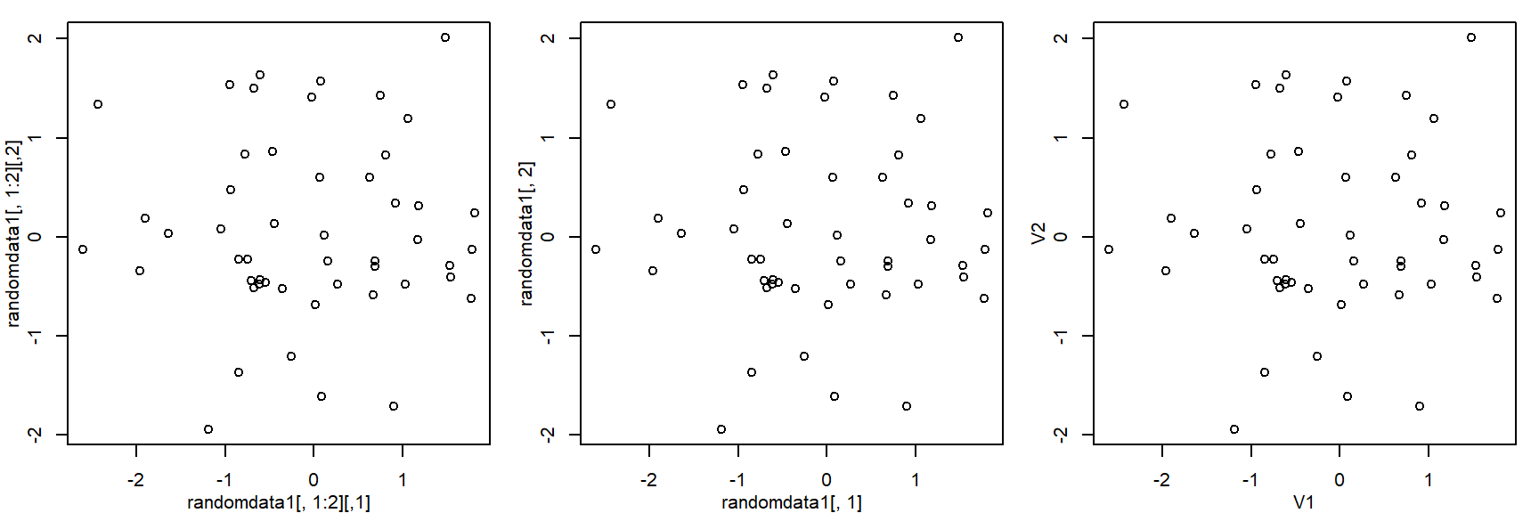
par(default_par)

# step 3 ----
rmeans <- colMeans(randomdata1)
rmeans
## [1] -0.05370906 0.05877590 -0.02721456 0.33318482 -0.06135820 -0.14629890
## [7] 0.05321337 0.03843854 -0.01410306 -0.22700718rsd <- apply(randomdata1,MARGIN=2,FUN=sd)
rsd ## [1] 1.1008056 0.9125635 1.0662123 0.8365269 0.8621626 0.9516279 1.1954454
## [8] 0.9414005 1.1403517 0.9765020# step 4 ----
boxplot(randomdata1[,1:2])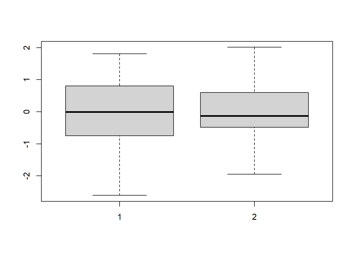
boxplot(list("First column"=randomdata1[,1],
             "Le Deux"=randomdata1[,2]))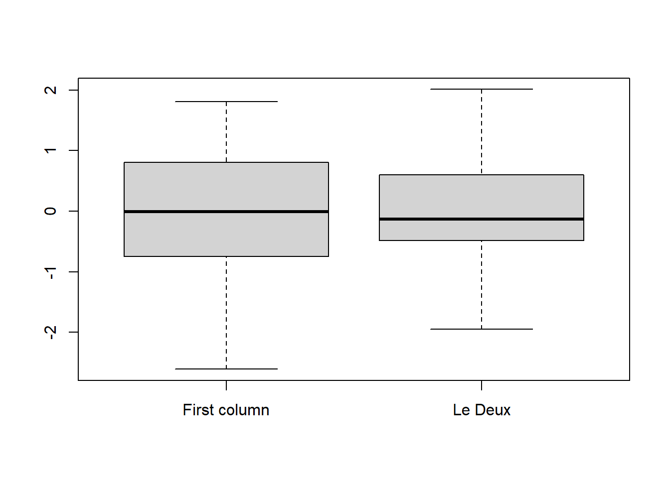
boxplot(randomdata1)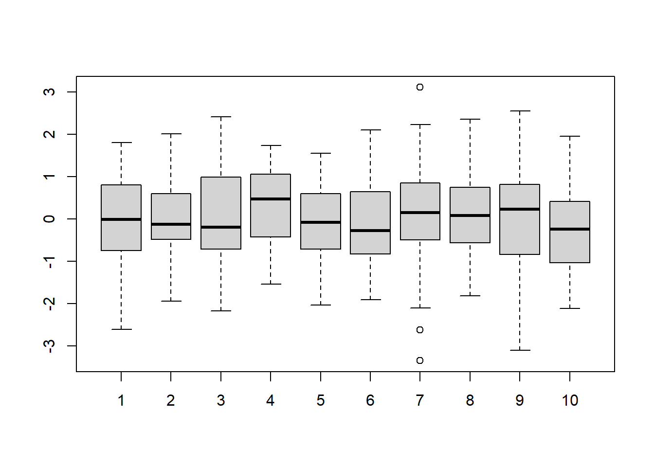
hist(randomdata1[,1])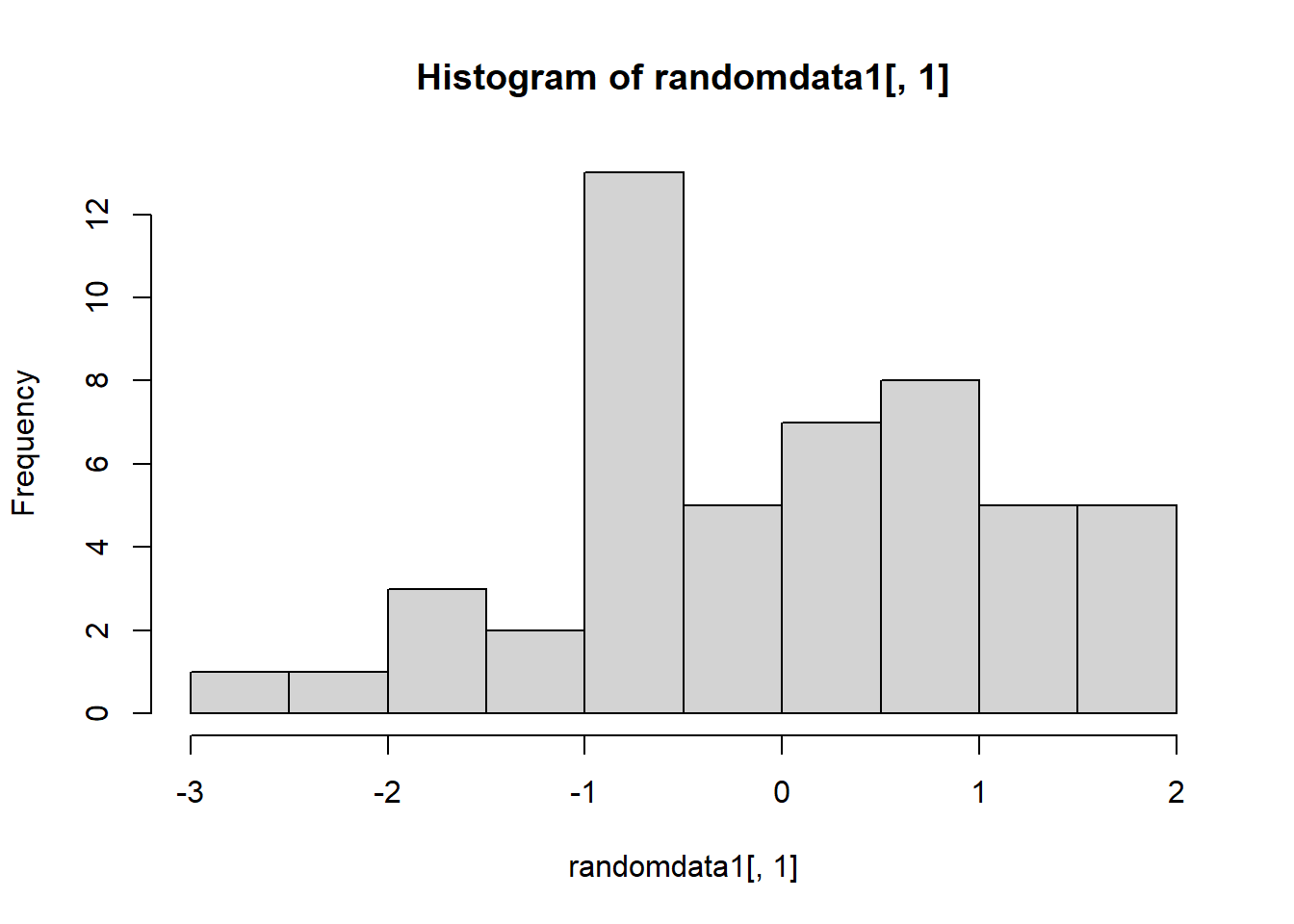
hist(randomdata1)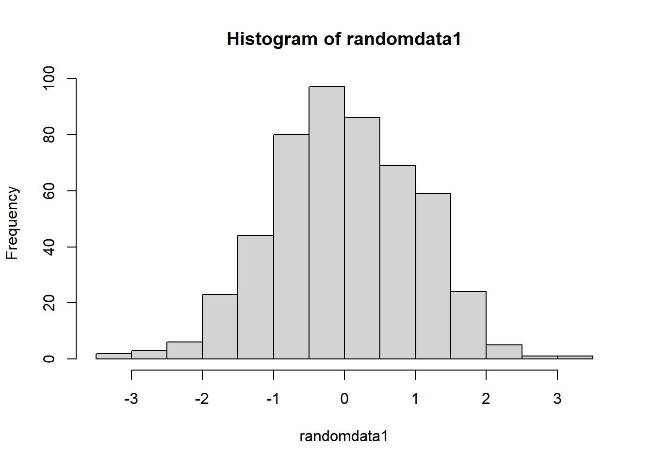
Assignment 4 notes
Do yourself and I a favour by submitted part 1 as an R script.I’ve read the assignment more closely, and it would be easier for me (and probably you) if you just submitted a text file with each answer (the RegEx or sentence response) on a line, so that I can easily copy and paste into my test code. Still best for you to write the text file in RStudio so that you know it won’t be converted to rich text, and you can easily test your RegEx.
- For part 2, remember that a FASTA file is a text file where each sequence is preceded by a header line that starts with
>. You can usereadLinesto read in the file as a character vector, then loop over it to either start a new sequence if you find>else append the line to the current sequence string.
- To clarify what part of each sequence you should be using: Each sequence in the FASTA file includes the preceding and following 1k base pairs. All we want you to store in the dataframe is the first 1000 base pairs of the sequence, and the last 1000 base pairs of the sequence. Don’t worry about finding the ORF start codon or anything like that, just paste the whole sequence together, then grab the substrings containing the first and last 1000 bp and paste them together in that dataframe. Note that when looking for the transcription factor binding sites, you should only look in the first 1000 bp, so you’ll have to substring the sequence again.
- Note that the final question wants a percentage per motif rather than per transcription factor in the
yeast_tf_motifs.txtfile. While some of the motifs in that file are ascribed to the same transcription factor, we expect a value per motif.